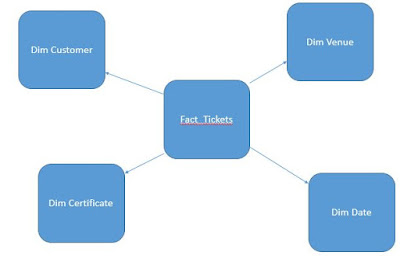
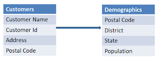
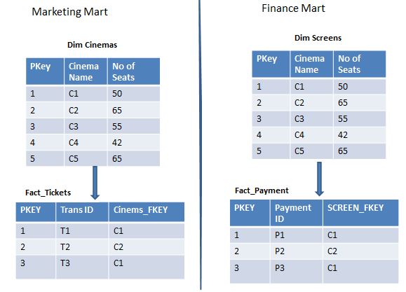
Saturday, September 8, 2018

Shrunken Dimension - Very useful for higher level summary

Shrunken Dimension is a very special type of dimension when there is a requirement of higher level of summary and lower grain data is already available in the warehouse.

Before we dive in if you do not understand what is the grain of the dimension, it is important to understand.

Month could be a shrunken dimension of date,  which could be connected to a fact which has grain of month like monthly sales. But this is a very classic example, let us deep dive a little with another example.
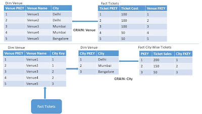
Considering the Online Movie Ticketing business scenario, we would have 2 tables, a fact for Ticket sales and a related dimension of the Venue for which sold the ticket. 
If customer need to view the total consolidated Sales at city level rather than Venue level, we could create a separate dimension for City and a separate fact table for Consolidated Sales. The image below demonstrates the same:
Shrunken Dimension Example

In the example above we have created a base dimension and Shrunken dimension separately. If needed we could also create the Shrunken dimension from the base dimension, once it is loaded. Again it totally depends on the business requirements and the type of source system you are dealing with.

Static Dimension in Datawarehouse

Static Dimension are not extracted from the data source, but created in warehouse itself in the context of warehouse. These are usually loaded just once, manually or by the help of a procedure. The data of this dimension does not change or changed very rarely.

A few common examples of the static dimensions would be "DIM_SOURCE_SYSTEMS", "DIM_STATUS_CODE" or date time as well.

Please do not confuse it with the SCD Type 0. In SCD type 0, we insert data regularly but never update it. Also, they are loaded with the data extracted from source.

Click here to read about the other dimensions in datawarehousing.

Sunday, September 2, 2018

Microsoft Teams is now Free - Can it be the Game Changer

Microsoft Teams is a platform that combines workplace chat, meetings, notes, and attachments. The service integrates with the company's Office 365 subscription office productivity suite, including Microsoft Office and Skype, and features extensions that can integrate with non-Microsoft products.

Microsoft initially released in 2017, but recently Microsoft announced a free version of it, which could be very useful for new startups or educational groups which want to collaborate for free with lots of features.

So what does the free version of Microsoft teams allows you to do:
  • Add up to 300 members to collaborate with 2GB free space per user.
  • 10 GB shared storage
  • Unlimited messaging and search.
  • Secure File Sharing
  • One on one Meetings with audio and video facilities.
  • Channel Meetings for Multiple People in team
  • Screen Sharing
  • MS word, PowerPoint, excel and One Note
  • Access to 140+ other apps and services
  • All this is available over cloud, which means it is not device specific. Just login with your account and you got all you work saved using other machines.

Sunday, August 19, 2018

What is Inferred dimension and Why it is important

Inferred Dimension, also referred to as Early coming Fact or Late coming dimension. These all are different names of same scenario.

If the source systems of your Data warehouse are very well designed, you should never face this scenario. But, sometimes it would happen that the fact data is available in the source but related dimension data does not yet exists.

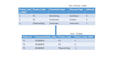
Consider that Online Movie Ticketing business scenario. Suppose a sales person sold some bulk movie tickets to an organisation at some discount. He provided a discount with a new promotion code, which he is supposed to punch in the system but forgot. When the ETL would process the data it will find that the promo code is not available.

There are 2 ways to handle this scenario:

  • 1st one is to mark the FKey as unknown. This is the simplest option but these sales records could not be used for the reporting purpose unless the dimension record arises or the fact is updated accordingly. Which is an ETL overhead altogether.
  • The other option is to use Inferred Dimension. For any such record we could create an entry in the dimension table and mark it inferred as shown in the image below.
Inferred Dimension
Using this method, our fact record could be used for reporting and a better picture would be generated. At a later load when the promo code details would be available, the dimension record could be updated automatically, depending on what type of Slowly Changing Dimension it is.

Sunday, August 12, 2018

OLTP vs OLAP explained

Both OLAP and OLTP are databases are designed for different purposes.

OLTP stands for Online Transaction Processing and is optimized for insert. update and delete operations. This is the reason these are used behind the application for regular business transactions.

OLAP stands for Online Analysis Processing and this databases are optimized for read operation and are widely used for analyzing, mining and reporting on large datasets.

It is important to note here that the database in which we store all the Facts and Dimensions is also OLTP. Post this we move the data to create a cube, which is stored in a OLAP database.

The image below explains the major differences of a OLTP and OLAP systems.
Now that we know the basic difference between OLTP and OLAP, lets now dig a little deeper.

  • The core of any OLAP system is a Cube, which is just a three-dimensional spreadsheet, where as in OLTP data is stored in 2D tables.
  • A cube consists of Numeric Facts called measures and are categorized by dimension data.
  • The metadata of any cube is star schema or Snowflake Schema or Fact Constellation in relational(OLTP) database. Measures are derived from the records in the fact table and dimensions are derived from dimension tables.
  •  While we can perform CRUD operation in OLTP, there are a few more operations which we could perform on a cube. These include Slicing, Dicing. Pivoting etc.

What is fact table in data warehouse

In data warehousing, a fact table consists of measurable entities of any business. It is surrounded by multiple dimensions in a star or snowflake schema.
In ideal scenario it has 2 types of columns:

  • Foreign Keys to the related dimension
  • Measurable columns like price etc.
It usually provides the calculative values(count, sum etc) which could be analysed across different dimensions. It is important to define the grain of each fact to the lowest level of reporting needs.


If we consider the Data-warehouse scenario of Online Ticket Booking, The first fact that comes to mind is for tickets.
So, if at any point of time business needs to find out how many tickets were sold for each cinema, they could simply join Fact_Tickets with Dim_Cinemas table as detailed in below image.
Fact


This suggests that 2 tickets were sold in cinema C1 and 1 ticket was sold for cinems C2

Different Operations on a OLAP cube in datawarehouse

The common operations on a cube are Slice, Dice, Drill-down, Roll-Up, pivot. These could be used individually or together to generate the desired picture of data.

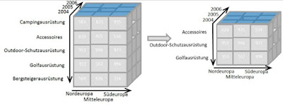
Slice is an act of picking a subset of the cube by choosing a single value for one of its dimensions. This create a new cube with fewer dimension.
The picture below shows a slicing operation:   The sales figures of all categories and all regions is sliced for just year 2004.
OLAP CUBE Slicing
Dicing allow the analysts to create and visualize a sub cube by selecting multiple values from multiple dimensions. The picture below shows dicing operation:
OLAP CUBE Dicing
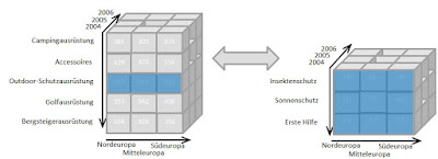
Drill down / up allows the analyst to navigate through the levels of data from most summarized to most detailed. The picture shows the drill down operation from summary category "Outdoor-Schutzausrüstung" to see the sales figures for the individual products.
OLAP CUBE Drill DOWN

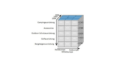
Roll Up means summarizing the data along a dimension. The summarization  could be calculating, count, total across a dimension hierarchy or more complex formulas like profit from sales etc. The picture below shows the summation of sale for each categories.
OLAP Cube Rollup

Pivot allows the analysts to rotate the cube in space to the desired direction, which gives the data and visualizations a totally different perspective. The image below show that.
OLAP Cube Pivoting


Sunday, August 5, 2018

Fact Constellation schema in Data warehousing

Fact Constellation: Fact Constellation allows you to connect multiple facts to dimensions. It is combination of multiple stars connected with each other using dimension, hence called Galaxy or Fact Constellation schema.

As compared to Star and snowflake it is used for more sophisticated application. The dimension tables could be normalized or not as per the requirement.

If you do not understand the basic concepts of data warehousing, please visit my previous article.

If we consider the data warehousing scenario detailed here, below is how is galaxy or fact constellation schema would look like.


Fact Constellation or Galaxy Schema

Characteristics of Fact Constellation schema:

  • Complex design
  • Different variants of aggregations
  •  Suitable for more sophisticate application 

Wednesday, August 1, 2018

Snowflake schema

Snowflake Schema: When one fact is surrounded by a chain of more than one dimension, it is called snowflake. It is also called an extension of star schema by adding more dimensions.
In snowflake schema the table are normalized.

If you do not understand the basic concepts of data warehousing, please visit my previous article.

If we consider the data warehousing scenario detailed here, below is how a snowflake schema would look like.

Snowflake Schema
Click here to compare the same design with star schema.

Characteristics of Snowflake schema:

  • Less storage requirement because of normalized dimensions
  • Less time to load as compared to star schema.
  • Better slicing and dicing
  • Join complexity increase
  • Time to Query may increase a little depending on the scenario.
Click here to learn more about different types of schema.

Star Schema - The simplest of all

Star Schema : It is simplest data warehouse schema. It is called star because it resembles the star with points radiating out of the center. Fact tables is the center of the star and dimensions sit at the points.
Usually the fact table in the star schema is in 3rd normal form and dimensions are usually de-normalized. It is most simplest and most commonly used schema.

If you do not understand the basic concepts of data warehousing, please visit my previous article.

If we consider the data warehousing scenario detailed here, below is how a star schema would look like.
Star Schema

Although, star schema require just one fact table at the center, but you could surely have multiple stars in your design.

Characteristics of  star schema

  • Simplest design
  • Better query performance.
  • A little extra time to load the data into dimension because of de-normalization.
  • More space because of redundancy in dimensions.
Click here to learn more about different types of schema.

Saturday, July 28, 2018

What is schema in Data warehousing and type of schemas

Definition: A schema is a collection of tables, views, indexes and synonyms. Each of these individuals are called schema objects. In simple terms terms we could say a schema is collection of database objects.

Schema plays a very important role when we design a data warehouse, because that would decide if the data warehouse we are building would serve its purpose. There are quite a few terminologies or types of schema. I am going to cover here a few which are very commonly used or reffered.

Before we get into that, it is important to note these are just design principles which are good to know but are not hard rules. Feel free to adapt as per your business requirements.

Commonly used schema types are:

Enumerating Datasets and Reports in Power Bi Tenant

Below is how you enumerate through the datasets and reports in a power bi tenant.
  1. Install the Power Bi Management cmdlts and login to your power bi
    Download the power bi Management cmdlts from here. click on the deploy button as shown in the image below and login using your Power Bi admin account
    Power BI admin Management cmdlts installation

    .
  2. Enumerate through all datasets that uses SQL server database
    Use the Get-PowerBIDataset and Get-PowerBIDatasource to the enumerate through the data sets. Below is how the power shell should look like:
    $datasetIds = Get-PowerBIDataset -Scope Organization -ErrorAction SilentlyContinue | Foreach {$dsId = $_.Id; Get-PowerBIDatasource -DatasetId $dsId -Scope Organization -ErrorAction SilentlyContinue | Where-Object {$_.DatasourceType -eq 'Sql' -and ($_.ConnectionDetails.Server -like 'sqldb01' -and $_.ConnectionDetails.Database -like 'DBNAME')} | Foreach { $dsId }}
  3. Enumerate all reports that use the identified datasets
    Using the dataset IDs found in the step 2, enumerate through the all the reports which are using the datasets
    $reports = $datasetIds | Foreach { Get-PowerBIReport -Filter "datasetId eq '$_'" -Scope Organization }

Friday, July 27, 2018

API and powershell for Power Bi Administrators

Power Bi enables organisation to be more data driven by empowering every business user build there own reports. But organisations must be capable to govern this self service BI boom. So the IT administrators must be capable of handling Licencing, Capacity, Security, Governance and Regulatory requirements.

To help achieve this, last week Microsoft released  APIs, power shell and .Net sdk for power bill admins.

A general scenario: Consider you have a database which is being used by many users and is under heavy load. Obviously there would some reports which could be optimised to reduce query size. As an admin if you could trace which are these reports you could then ask the users to optimise. This can be achieved by enumerating through resources under your tenant. Click here to read about how can we enumerate and identify.

This is just one example, but you could achieve a lot more. Below are some more related resources.

https://docs.microsoft.com/en-us/powershell/power-bi/overview?view=powerbi-ps
https://github.com/Microsoft/powerbi-powershell
https://github.com/Microsoft/PowerBI-CSharp
https://docs.microsoft.com/en-us/rest/api/power-bi/
https://docs.microsoft.com/en-us/power-bi/service-admin-reference

Thursday, July 26, 2018

Make all SharePoint Surveys truly anonymous real quick

If you have worked withe surveys, you must be knowing survey provide an option "Show user names in survey results", to make survey anonymous, If not you could refer this. Now the problem with this is anyone with rights to edit list settings could change this setting and all users would be visible. 

There is no suggested approach to do this there are lots of options available. One very nice article is available on this msdn blog. Mostly suggested changing the name using event receiver or workflows. But none of these serve my purpose, as i needed to make all the surveys on the farm anonymous including the new ones. Also with hundreds of surveys across the farm, these workflows or event receivers could hamper performance.
So, i did a small trick to make sure no one to change the list setting and rest SharePoint could handle automatically.
I made some tweaking in the application page witch impacted all my surveys. We could also do the same for a particular site.
We will have to make changes in two application pages, available in layouts folder of 15 hive. Combined these changes will give an effect to of no in survey setting.
  1. ListGeneralSettings.aspx : This page opens when we click "ListName, Description, Navigation in site settings.
  1. New.aspx : This page opens when we create a new survey list. Page URL is same for both popup and advanced options page.
  1. To make sure user can not select yes on advanced options screen. To do this find the below ts tag and comment it.
  1. <td class="ms-authoringcontrols" nowrap="nowrap"><input id="onetidShowUserNamesNo" type="radio" value="on"  name="showUsernames" title="<SharePoint:EncodedLiteral runat='server' text='<%$Resources:wss,lstsetng_showusernamesyes_title%>' EncodeMethod='HtmlEncode'/>" /><label for="onetidShowUserNamesYes"><SharePoint:EncodedLiteral runat="server" text="<%$Resources:wss,lstsetng_showusernamesyes_label%>" EncodeMethod='HtmlEncode'/></label></td>
  1. By pass the Basic creation popup and navigate to advanced screen because by default SharePoint consider it yes. To do this:
  1. Find the below code in the file:
x


ListGeneralSettings:
Search for "Survey Settings" and make radio button with id "RADShowUserYes" hidden by adding attribute visible:false. This will hide the yes option in List settings.

New.aspx: We will make two changes in this file.
if (this.IsDialogMode){
    %><a class="ms-textSmall" href="javascript:;" onclick="NavigateToFullPage()"><SharePoint:EncodedLiteral runat="server" text="<%$Resources:wss,lstsetng_advancedoptions_text%>" EncodeMethod='HtmlEncode'/></a><%}

    and another if condition inside this if. Final code should look like this:

    if (this.IsDialogMode)
    {
    if (HttpContext.Current.Request.Url.AbsoluteUri.Contains("ListTemplate=102"))
            {
                Page.ClientScript.RegisterStartupScript(this.GetType(), "CallMyFunction", "NavigateToFullPage()", true);
            }else { 
    %>
    <a class="ms-textSmall" href="javascript:;" onclick="NavigateToFullPage()"><SharePoint:EncodedLiteral runat="server" text="<%$Resources:wss,lstsetng_advancedoptions_text%>" EncodeMethod='HtmlEncode'/></a>
    <%
            }}

    If you have any existing survey lists, you could use powershell to to change their list setting.

    How to Enable Share-point Designer in Central Admin

    Below are steps for SharePoint Designer settings in Central Admin:

    1. Open Central Application Website.
    2. Open SharePoint Designer Settings under General Application Settings.
    3. Select your web application from the drop down at the top of the form.
    4. Select the appropriate options as mentioned below(per your needs) and click  ok.
    There are four check boxes as listed below:

    Enable SharePoint Designer : This Enables or disables SharePoint Designer for the Web Application and all of its site collections.

    Note: If unchecked, users still see SharePoint Designer buttons in the browser, but when they click them, they get a message stating that SharePoint Designer is not allowed on the site.

    Enable Detaching Pages from the Site Definition : This option enables or disables the ability to detach pages from the site definition. If unchecked, SharePoint Designer only allows you to edit pages in normal mode. The Edit File in Advanced Mode is disabled. Running in Advanced mode lets a user ghost pages by modifying them from the content originally in the site definition stored on the server’s hard drive. The customized version of the page is stored in the SharePoint content database. Any changes made to the site definition files aren’t reflected in detached pages. This can create maintainability problems and should be used with care.

    Note: This setting does not apply to pages that have already been detached as well as new blank ASPX or HTML pages created by the user.

    Enable Customizing Master Pages and Layout Pages : This enables or disables the ability to customize master pages and page layouts. If unchecked, SharePoint Designer does not display Master Pages or Page Layouts in the Navigation pane.

    Note: Page layouts also require publishing enabled on the server, so if you have enabled it here but the site is not a publishing site, you will still not see the Page Layouts option in the Navigation pane.

    Enable Managing of the Web Site URL Structure: This enables or disables the ability to view and edit files in the URL structure of a site. If unchecked, SharePoint Designer does not display the All Files option in the Navigation pane.


    Note: These four options are also available at site collection settings.

    Sunday, July 22, 2018

    Bridge Tables in datawarehouse

    As the name suggests, bridge table is used to link tables when direct linking does not make sense. Usually used in a little complecated senarios when we have many to many relations between 2 tables.
    Example: Consider we have multiple customer linked to a single bank account balance. Putting multiple customer keys in that fact would create obvious problems in the fact table. 

    Bridge table is also used sometimes to manage variable hierarchies. For e.g. to maintain one primary customer and one or more secondary customers.

    Bridge table come to rescue in such situation, but just like outrigger dimension don't use it too much. Remember, every query has to pay toll to navigate the bridge.

    Although, it is not a dimension but I personally call it Bridge dimension because it has many properties of a dimension.

    Click here to read about the other dimensions in datawarehousing.

    Tuesday, July 17, 2018

    What is Outrigger Dimension and its purpose

    Definition:  As per Kimball, when in dimension in the DWH is linked with another dimension table, the secondary table is call outrigger dimension. For example a customer dimension referring to the Date dimension for the date of account creation.

    Now, it might seem like snowflaked(not complete), but it is not. There are a few differences as detailed below:

    • Snowflake make the structure highly normalized where as outrigger makes it partially normalized.
    • Snowflake makes the ETL complicated and reduces the query performance.
    While, Now outrigger dimensions are similar to snowflake but are vary limited in nature. They are just one or more levels removed fro the fact table. This is mostly used when there is a business requirement to slice and dice of the particular column. 

    Consider the following criteria before creating an outrigger dimension:
    • User Analytics Needed: If the user wants to slice and dice on the column
    • Data Granularity vs Cardinality : A column with high low granularity and high cardinality is a candidate.
    • Update Frequency : If a column is updated very frequently, not more than once a month
    • It is divided in the source itself.
    • Customer and it location would be a good candidate for outrigger dimension
    Outrigger Dimension

    For list of dimensions in data-warehouse, click here

    Granularity and Cardinality of a table

    What is granularity : Granularity is the measure of grain for any table. Facts are usually designed at the lowest level of granularity, such that we can trace the lowest level of details when needed.

    What is Cardinality : Opposite to Granularity, cardinality is calculated at the column level. Cardinality refers to the number of  unique values a table has.  For example in a customer table Customer Name would have higher cardinality than location, whereas Customer ID would have the highest cardinality of one or 100 %.

    Wednesday, July 11, 2018

    Generic DateTime dimension - Part 2

    In Part 1 of this post blog i talked about a generic dimension for Date, which is pretty simple and effective.

    Continuing from there, below are the Calculation for each field:


    1. [DATE_PKEY]  AS (CONVERT([int],CONVERT([char](8),[DATE],(112))))
    2. [DAY_OF_MONTH]  AS (datepart(day,[DATE]))
    3. [DAY_SUFFIX]  AS (case when datepart(day,[DATE])=(13) OR datepart(day,[DATE])=(12) OR datepart(day,[DATE])=(11) then CONVERT([varchar],datepart(day,[DATE]))+'th' when right(datepart(day,[DATE]),(1))=(1) then CONVERT([varchar],datepart(day,[DATE]))+'st' when right(datepart(day,[DATE]),(1))=(2) then CONVERT([varchar],datepart(day,[DATE]))+'nd' when right(datepart(day,[DATE]),(1))=(3) then CONVERT([varchar],datepart(day,[DATE]))+'rd' else CONVERT([varchar],datepart(day,[DATE]))+'th' end)
    4. [DAY_NAME]  AS (datename(weekday,[DATE]))
    5. [DAY_OF_WEEK]  AS (datepart(weekday,[DATE]))
    6. [DAY_OF_QUARTER]  AS (datediff(day,dateadd(quarter,datediff(quarter,(0),[DATE]),(0)),[DATE])+(1))
    7. [DAY_OF_YEAR]  AS (datepart(dayofyear,[DATE]))
    8. [WEEK_OF_MONTH]  AS ((datepart(week,[DATE])-datepart(week,dateadd(month,datediff(month,(0),[DATE]),(0))))+(1)),
    9. [WEEK_OF_QUARTER]  AS (datediff(week,dateadd(quarter,datediff(quarter,(0),[DATE]),(0)),[DATE])+(1))
    10. [WEEK_OF_YEAR]  AS (datepart(week,[DATE]))
    11. [MONTH]  AS (datepart(month,[DATE]))
    12. [MONTH_NAME]  AS (datename(month,[DATE])),
    13. [MONTH_OF_QUARTER]  AS (case when datepart(month,[DATE])=(10) OR datepart(month,[DATE])=(7) OR datepart(month,[DATE])=(4) OR datepart(month,[DATE])=(1) then (1) when datepart(month,[DATE])=(11) OR datepart(month,[DATE])=(8) OR datepart(month,[DATE])=(5) OR datepart(month,[DATE])=(2) then (2) when datepart(month,[DATE])=(12) OR datepart(month,[DATE])=(9) OR datepart(month,[DATE])=(6) OR datepart(month,[DATE])=(3) then (3)  end),
    14. [YEAR]  AS (datepart(year,[DATE])),
    15. [YEAR_NAME]  AS ('CY '+CONVERT([varchar],datepart(year,[DATE]))),
    16. [MONTH_YEAR]  AS ((left(datename(month,[DATE]),(3))+'-')+CONVERT([varchar],datepart(year,[DATE])))
    17. [MMYYYY]  AS (right('0'+CONVERT([varchar],datepart(month,[DATE])),(2))+CONVERT([varchar],datepart(year,[DATE])))
    18. [FIRST_DAY_OF_MONTH]  AS (CONVERT([date],dateadd(day, -(datepart(day,[DATE])-(1)),[DATE])))
    19. [LAST_DAY_OF_MONTH]  AS (CONVERT([date],dateadd(day, -datepart(day,dateadd(month,(1),[DATE])),dateadd(month,(1),[DATE]))))
    20. [FIRST_DAY_OF_QUARTER]  AS (CONVERT([date],dateadd(quarter,datediff(quarter,(0),[DATE]),(0))))
    21. [LAST_DAY_OF_QUARTER]  AS (CONVERT([date],dateadd(quarter,datediff(quarter,(-1),[DATE]),(-1))))
    22. [FIRST_DAY_OF_YEAR]  AS (CONVERT([date],dateadd(year,datediff(year,(0),[DATE]),(0))))
    23. [LAST_DAY_OF_YEAR]  AS (CONVERT([date],dateadd(year,datediff(year,(0),[DATE])+(1),(-1))))
    24. [CALENDER_YR_QUARTER]  AS (datepart(quarter,[DATE]))
    25. [FINANCIAL_YR_QUARTER]  AS (case datepart(quarter,[DATE]) when (1) then (4) when (2) then (1) when (3) then (2) when (4) then (3)  end)
    26. [FINANCIAL_YEAR]  AS (case datepart(quarter,[DATE]) when (1) then (CONVERT([varchar],datepart(year,[DATE])-(1))+'-')+CONVERT([varchar],datepart(year,[DATE])) when (2) then (CONVERT([varchar],datepart(year,[DATE]))+'-')+CONVERT([varchar],datepart(year,[DATE])+(1)) when (3) then (CONVERT([varchar],datepart(year,[DATE]))+'-')+CONVERT([varchar],datepart(year,[DATE])+(1)) when (4) then (CONVERT([varchar],datepart(year,[DATE]))+'-')+CONVERT([varchar],datepart(year,[DATE])+(1))  end)

    Generic DateTime dimension in data warehouse

    If you have worked on a data warehouse you would surely have a dimension for Date. It is usually called Dim_Date, Dim_Time or Dim_DateTime. Don't get confused by the use of word time, the table is usually create with grain of one day unless there are some very specific reporting requirements.
    So what should be columns in this dimension and how it should be populated and maintained. From my experience in datawarehousing, i have created a generic dimension for date which works in almost all scenarios and is does not require any maintainance.
    Below is how the structure looks like.

    As you could notice apart from the first column, rest of the columns are Computed. So by using this approach we need not to create any ETL for it and hence no maintenance pain.
    At the moment there are 27 columns in the table above but you can surely add more as needed.

    All we need to do is populate the first column with a simple SQL query and rest of the columns will follow.

    Below query inserts the dates in the table from year 2010 to year 2022. You could update the dates as per your need

    declare @start_date datetime, @end_date datetime, @cur_date datetime
    set @start_date = '2010-01-01'
    set @end_date = '2022-12-31'
    set @cur_date = @start_date
    while @cur_date <= @end_date
    begin
    insert into [Dim_Date](Date)
    select CONVERT(varchar, @cur_date) as Date
    set @cur_date = dateadd(dd, 1, @cur_date) 
    end

    Formulas of the computed fields are available here.

    What is grain of a table in data warehousing

    In simple terms grain is the lowest level till which you could identify the data in a table.
    For example: If you have table which holds the stock inventory and table holds:

    1. One record for each day of the stock : Than the grain would be one day
    2. One record for each hour : than the grain of the table would be hour
    3. One record for each week : than the grain of the week would be week.


    How does grain impacts the data warehouse:
    It is important that while designeing the databse we design till the lowest grain for which we business needs to analyse or report.
    With example above, If your Stock inventory table has grain of day you can easily calculate weekly stock but viceversa is not true.

    Similarly, grain of related tables(Facts and Dims) should complement each other. For eg if Fact_Stock_Inventory holds data for each hour and Dim_DateTime has a grain of a day, it will generate distorted results.

    Tuesday, July 10, 2018

    What is Conformed Dimension and its advantages

    People usually finds it difficult to understand the Conformed dimension, I am trying to explain it with an example. To start with, please do not confuse it confirmed / static dimension, because of the name.

    Definition: A conformed is defined as a dimension, which has the same meaning to all the facts in a data warehouse, even if the facts belong to different data-marts.
    It could one single table or multiple copies of same table across different marts. There is no hard rule  of the copies having the same table name. One copy could even be a sub set of another copy.

    Let us now try to understand it with a example. Consider online movie tickets data warehouse scenario.
    Lets assume we have divided our EDW into 2 data marts

    • Marketing : Marketing team is more concerned about the no of tickets sold.
    • Finance : Finance team is more concerned about the profit.


    Both teams would require to know the stats for each cinema. Now, both teams might also have different terminologies. Marketing team might call it Cinems whereas finance team might call it Screen.
    So in this scenario we could create 2 copies of same table with different names as shown below.
    Confirmed dimension explained


    But why should we use it. Why don't we create 2 separate tables if we need. Below are a few disadvantages of not creating Conformed dimensions:

    • There will more ETL work to generate the logic of different tables.
    • More ETL will surely mean some extra maintenance effort.
    • and possible difficulties in joining multiple data marts. 

    Visit my post on Types of Dimensions to understand more about different types of dimensions.

    Monday, July 9, 2018

    List of dimensions in a Data Warehouse

    Below is the list of dimensions types we should consider while designing any data warehouse. Click on the link below for a detailed definition and example.


    This list will keep on improving with time, so you can bookmark this page and  feel free to subscribe to the blog by entering your email

    What is Enterprise data warehouse or EDW

    Wikipedia says, a data warehouse (DW or DWH), also known as an enterprise data warehouse (EDW), is a system used for reporting and data analysis, and is considered a core component of business intelligence.
    DWs are central repositories of integrated data from one or more disparate sources. They store current and historical data in one single place that are used for creating analytical reports for workers throughout the enterprise.
    EDW can be logically divided into the data-marts depending on business areas like HR, Finance, Production etc. It is important to note that a data-mart is just a logical divide and you could still hold the data together physically

    Below are major components of the any data warehouse:
    1.) Date warehouse tables which include Facts and Dimensions. These are stored in a OLTP database.
    2.) OLAP or Cube for reporting
    3.) ETL Tools

    Sunday, July 8, 2018

    What is a dimension in data warehouse

    As per Wikipedia, A dimension is a structure that categorizes facts and measures in order to enable users to answer business questions.
    Commonly used dimensions are people, products, place and time.

    If we consider the Data-warehouse scenario of Online Ticket Booking, The first dimension that comes to mind is for List of cinemas.
    So, if at any point of time business needs to find out how many tickets were sold for each cinema, they could simply join Dim_Cinemas with tickets table as detailed in below image.


    This suggests that 2 tickets were sold in cinema C1 and 1 ticket was sold for cinems C2

    There are many types of dimension in a data warehouse listed here.

    Friday, July 6, 2018

    Windows 7 is dangerous to use, Warns Microsoft

    Microsoft recently published a post(in German) warning customers to move from Windows 7 to windows 10. The official new room warns that the ageing platform suffers from various failings including security issues and lack of hardware support.
    Microsoft further added that windows 7 has an outdated security architecture, and people using it are more susceptible to cyber attacks.

    Is there a real threat or it is just a scare tactic

    • Let me say it clearly, Windows 7 is totally safe and users should not panic. Is seems like a desperate attempt to push people to upgrade.
    • Provided, system is upgraded with latest updates, you their is nothing to worry.
    • Windows 7 supports ends officially in 2020, so you have ample time to move at your pace for upgradation.

    Conclusion: windows 10 security architecture is better than windows 7, but there is no hurry to upgrade. Windows 7 was one of the best version of Windows, so you can comfortably take your time de-addict your self.

    What is Junk Dimension and its purpose

    Definition: By definition, it is a collections of random transnational code flags. It is usually created by joining multiple low cardinality dimensions into one.
    As we merge different dimensions in to one, it will reduce the number of foreign keys in the fact table.

    If we consider the Data warehouse scenario of Online Ticket Booking, The design should have following 3 tables, with fact having 2 foreign keys one for each dim.

    • Fact_Tickets
    • Dim Transaction Type
    • Dim Cert Type

    Both Dims are of very low cardinality(i.e. no of records in each dim would be very low)
    Transaction Type : The values could be Net-banking, Card, Wallet. The chances of increasing this count is very low
    Movie Certificate : The values could be U, A, U/A. Again the chances of increasing/Changing these is very rare.

    The picture below describes the 2 possible designs of it, if  we keep these parameters in dimension table.
    Junk dimension


    So with the help of junk dimension, we converted 2 forein keys in to one.
    No of Records: Notice that, the no of records in the junk transaction is the multiplication of no of records in each dimension. In the example above there are 3 records for both Transaction and Certificate, so the total count in junk dimension is 9.
    If we are merging 3 tables with 3 records each, the no of records in the junk dimension would be 27(3*3*3)

    Ensure the dimensions we junk together should be of very low cardinality. I would suggest the no of records in the junk transaction should be less than thousand.

    Please feel free to post your queries in the comments section and follow this blog.

    Data-warehouse scenario - Online ticket Booking Business

    I am writing a series of articles on Data warehousing design concepts. During the series i will use the following scenario in all my examples.

    Scenario: Consider we are building a warehouse for a company which sells Online\Offline movie tickets. For e.g. BookMyShow in India and Movie Tickets in USA or UK.

    The major business areas of would be:
    • Customer
    • Movie Details
    • Ratings
    • Tickets
    • Transactions
    • Venues
    • Cinemas
    • Promotional Codes
    • Will add more to this list as the series grows

    Wednesday, July 4, 2018

    Truncate Microsoft SQL Database without manually dropping Key constraints

    We all have faced times when we want to truncate all the tables of a database, but to truncate a table we need to drop the all the constarints. It is painful to drop all constraints, than truncate and recreate the constarints.
    If it is a small database this trick might work but for a big database it is next to impossible, specially when your database structure is changing over time.
    Although there is no out of the box way to do it, but with a few line of code we could surely do it.

    Following peice of code would do the trick. We can also create a procedure for it if needed regularly.

    We will need 3 tables to store the data temporarily. Let's first check if they already exists:
    IF OBJECT_ID('dbo.DropFkey', 'U') IS NOT NULL
        DROP TABLE dbo.DropFkey;
    IF OBJECT_ID('dbo.DROPTruncate', 'U') IS NOT NULL
        DROP TABLE dbo.DROPTruncate;
        IF OBJECT_ID('dbo.CreateConstraints', 'U') IS NOT NULL
        DROP TABLE dbo.CreateConstraints;

    Next step is to create a list of all the primary keys and store it into a table.
    ;WITH cte(consColumn,
             foreignKeyName,
             parentSchema,
             parentTableName,
             parentColName,
             refSchema,
             refTableName,
             refColName)
         AS (SELECT fkc.constraint_column_id AS consColumn,
                    fk.NAME AS foreignKeyName,
                    parentSchema.name AS parentSchema,
                    parentTable.NAME AS parentTableName,
                    parent_col.NAME AS parentColName,
                    refSchema.name AS refSchema,
                    refTable.NAME AS refTableName,
                    ref_col.NAME AS refColName
             FROM sys.foreign_keys fk
                  INNER JOIN sys.foreign_key_columns fkc ON fk.object_id = fkc.constraint_object_id
                  INNER JOIN sys.tables parentTable ON parentTable.object_id = fkc.parent_object_id
                  INNER JOIN sys.schemas parentSchema ON parentSchema.schema_id = parentTable.schema_id
                  INNER JOIN sys.columns parent_col ON fkc.parent_column_id = parent_col.column_id
                                                       AND parent_col.object_id = parentTable.object_id
                  INNER JOIN sys.tables refTable ON refTable.object_id = fkc.referenced_object_id
                  INNER JOIN sys.schemas refSchema ON refSchema.schema_id = refTable.schema_id
                  INNER JOIN sys.columns ref_col ON fkc.referenced_column_id = ref_col.column_id
                                                    AND ref_col.object_id = refTable.object_id
                                                    AND parentTable.type = 'U'
                                                    AND refTable.type = 'U')
         SELECT DISTINCT
                foreignKeyName,
                parentSchema,
                parentTableName,
                SUBSTRING(
                         (
                             SELECT ','+a.parentColName+''
                             FROM cte a
                             WHERE a.foreignKeyName = c.foreignKeyName
                             ORDER BY a.consColumn
                             FOR XML PATH('')
                         ), 2, 200000) AS parentColName,
                refSchema,
                refTableName,
                SUBSTRING(
                         (
                             SELECT ','+b.refColName+''
                             FROM cte b
                             WHERE b.foreignKeyName = c.foreignKeyName
                             ORDER BY b.consColumn
                             FOR XML PATH('')
                         ), 2, 200000) AS refColName
        INTO #FkeyDesc
         FROM cte c;

    Now that we have the list of all the foreign keys, we can drop the keys in the table. We would use the list of keys stored above to re-create the keys post truncation.
    SELECT DISTINCT Row_Number() OVER ( ORDER BY foreignKeyName ASC ) AS RN,
           'IF  EXISTS 
        (SELECT * FROM sys.foreign_keys 
    WHERE 
    object_id = OBJECT_ID(N''['+parentSchema+'].['+foreignKeyName+']'') 
    AND 
    parent_object_id 
    = OBJECT_ID(N''['+parentSchema+'].['+ParentTableName+']''))
    ALTER TABLE ['+parentSchema+'].['+ParentTableName+'] 
    DROP CONSTRAINT ['+foreignKeyName+']' AS foreignKey_drop_script
    INTO DropFkey
    FROM #FkeyDesc;
    DECLARE @Job NVARCHAR(MAX);
    DECLARE @RN INT;
    DECLARE @RN1 INT;
    SELECT TOP 1 @Job = foreignKey_drop_script,
                 @RN = RN
    FROM DropFkey
    ORDER BY RN;

    WHILE @RN IS NOT NULL
        BEGIN
            EXEC sp_executesql
                 @Job;
            SET @RN1 = @RN;
            SELECT TOP 1 @Job = foreignKey_drop_script,
                         @RN = RN
            FROM DropFkey
            WHERE RN > @Rn1
            ORDER BY RN;
       IF @@ROWCOUNT = 0
            BREAK
        END;


    As the keys are dropped we could simply truncate all the tables, with the exception of tables which stores the list of keys to be regenerated
    SELECT DISTINCT ROW_NUMBER () OVER  (ORDER BY Name) AS RN,
    ' TRUNCATE TABLE '+ Name + '' AS TruncateScript
    INTO DROPTruncate
    FROM sys.tables
    WHERE type_desc = 'USER_TABLE'
    AND NAME NOT IN
    (
    'DropFkey',
    'DropTruncate',
    'CreateConstraints'
    --If neede we can add more tables here and these tables would not be truncated.

    DECLARE @RNTruncate INT;
    DECLARE @RNTruncate1 INT;
    DECLARE @JobTruncate NVARCHAR(MAX);
    SELECT TOP 1 @JobTruncate = TruncateScript,
                 @RNTruncate = RN
    FROM DROPTruncate
    ORDER BY RN;
    WHILE @RNTruncate IS NOT NULL
        BEGIN
            EXEC sp_executesql
                 @Jobtruncate;
            SET @RNTruncate1 = @RNTruncate;
            SELECT TOP 1 @JobTruncate = TruncateScript,
                         @RNTruncate = RN
            FROM DROPTruncate
            WHERE RN > @RNTruncate1
            ORDER BY RN;      
            IF @@ROWCOUNT = 0 BREAK;
        END;


    Now that all the tables are truncate we could simply re-create the keys.
    SELECT DISTINCT
            ROW_NUMBER () OVER  (ORDER BY foreignKeyName) AS RN,
           'ALTER TABLE ['+parentSchema+'].['+ParentTableName+']  WITH CHECK 
    ADD  CONSTRAINT ['+foreignKeyName+'] FOREIGN KEY('+parentColName+')
    REFERENCES ['+refSchema+'].['+refTableName+']('+refcolname+')' AS Add_constraints_script
    INTO CreateConstraints
    FROM #FkeyDesc; 
    DECLARE @RNCREATE INT;
    DECLARE @RNCREATE1 INT;
    DECLARE @JobCREATE NVARCHAR(MAX);
    SELECT TOP 1 @JobCREATE = Add_constraints_script,
                 @RNCREATE = RN
    FROM CreateConstraints
    ORDER BY RN;
    WHILE @RNCREATE IS NOT NULL
        BEGIN
            EXEC sp_executesql
                 @JobCREATE;
            SET @RNCREATE1 = @RNCREATE;
            SELECT TOP 1 @JobCREATE = Add_constraints_script,
                         @RNCREATE = RN
            FROM CreateConstraints
            WHERE RN > @RNCREATE1
            ORDER BY RN;
            IF @@ROWCOUNT = 0 BREAK;
     END

    Performance: It seems like a gigantic piece of code, but i have tested it on database with more than 100 tables and a few million records. Execution time was approx 1 minute.

    Feel free to post your queries in comments and follow this blog if you liked the post.
    Tuesday, July 3, 2018

    How to import large SQL files in database

    I recently faced an situation, where i was supplied with a .SQL file which was exported from a large table with some million records. The file was exported from the generate script options of SSMS and  had the insert statements. The size of the file was more than 2GB.

    SSMS(SQL Server Management Studio) is not capable enough of handling such big files. It would through one following error:

    • Insufficient memory to continue the execution of the program.
    • or SSMS would simply reject the request to open the file.

    SQLCMD is the life saver here. We could use SQL command line utility to execute the T-SQL commands. It is pretty simple to use as detailed below:

    1. Open the Command prompt with the administrator privileges.
    2. Execute the following command.

    
     sqlcmd -S SQLSERVER\InstanceName -i "F:\File.sql"


    The difference: SSMS uses the .Net framework for execution where as the command line uses ODBC driver.

    Thursday, June 28, 2018

    ETL or ESB : What is better fit for your design

    I have often seen people getting confused about, what would be a better fit for movement of data in their system. Their is a lot of content out their about these two technologies. Today i am trying to elaborate these in a very basic example.

    Domino's(The pizza giant) logistics is a very good example to understand.
    So how domino's works:
    They prepare their dough, veggies, spices etc. in their factories than big giant trucks supply these materials to their outlets once or twice a day.

    This is what ETL is. Scheduled movement of large quantity data from source to destination. Obviously in real scenario we do some data transformations in between.

    The outlets usually have their delivery bikes to deliver the order in smaller chunks as they receive the order. This is ESB. Delivery of small chunks of data to the needy system in near real-time manner.

    Would it make sense to use a large truck to deliver the pizzas only once or twice day or vice versa. This will not work at all. This is why it is important plugin in the right component in the system.

    I hope i explained it well. Let me know if you have any questions?

    Monday, June 18, 2018

    Checksum - How to find incremental data when there are no dates column in the source, using Talend DI

    I recently came across a situation where we needed to perform incremental on some data, but the problem we cam across is that there was no date column in the source feed which could help us find the incremental data.
    When you have an insert date and update in the source you could simply filer the data of source using the date column. We could surely find out the the new inserts by comparing the business keys but to find out the updates one need to compare each column value. This would make the performance very bad if there many columns in the table.

    Scenario:
    Suppose we have an employee table in the both source and target table with some 20 columns. Now comparing each column of the table in both source and target db for each row could not be a solution. We decided to generate the checksum for each row in the data and compare the checksum values for each row.
    What is Checksum: Checksum is an error detecting algorithm and it generates a unique number for a string provided. There are multiple algorithms to generate checksum and we used CRC32.

    I am demonstrating this in Talend, but one could use almost any ETL tool to replicate the same.
    For the purpose of demonstration , let us take 3 columns:

    • EmpId(PK)
    • Name(Changing Attr)
    • Salary(Changing Attr)


    Table Employee source has these 3 columns. The table Employee Target would have same structure with one extra column name checksum. Consider the snapshot below to understand the data.


    Below is how the talend job looks like.
    Talend job for checksum

    It reads the data from source employee table and the java code in the component "tJavaRow" adds another column named checksum to the flow. Below is how the java code looks like.
    output_row.EmpID = input_row.EmpID;
    output_row.Name = input_row.Name;
    output_row.Salary = input_row.Salary;
    String rowConcat= input_row.EmpID+input_row.Name+input_row.Salary;

    CRC32 crc = new CRC32();
    crc.update(rowConcat.getBytes());
    output_row.Checksum=Long.toString(crc.getValue());

    Here we have concatenated all the 3 columns and calculated the checksum on it. Please note that the sequence of column is important.

    After that tMap is comparing the checksum value generated in the process and checksum value already available in the target table.

    As seen in the out put below, one row went to the insert branch and 1 row went to the update branch.The log window below shows the checksum values generated.

    If you liked the post, please share it.
    Subscribe to your email and receive new articles on your email